Introduction

We live in the era of information overload, we consume massive amounts of information from different sources in a daily basis, but how do we find interesting stuff inside these information? How do we discover an interesting book out of the millions of books available in Amazon? How do we chose a nice pair of shoes out of the hundreds of thousands in Zalando? An interesting book for me might be a boring book for you, and a particular pair of shoes that is cool for me might be not your taste. Recommender Systems deal with problems like that, such a system uses previous purchases and user interaction to prescribe the user with items that most likely she would like to consume.

The core problem of recommender systems is to estimate a utility function that would predict how much a user would like an item, such a function takes into consideration previous purchases, user-site interaction, user-user interaction, item similarity based on their content, the context of a specific user session and other attributes.

Collaborative filtering

A popular algorithm that uses only previous purchases/behavior is collaborative filtering. On the collaborative filtering setting we have n user, m items and r ratings, those ratings can be collected either explicitly (e.g. stars in Amazon) or implicitly from user behavior (e.g. purchasing an item is better rating than putting it on the wish list which is better than just clicking the item without further actions). This kind of information is represented in a user-item matrix similar to the following example :

 

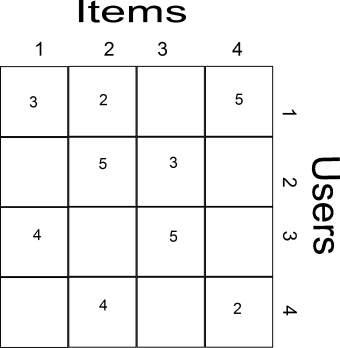
This matrix is a sparse matrix because not all users had rated all items. The aim of a recommender system is to fill this matrix. In collaborative filtering the items are modeled as vectors of the user ratings, therefore by using a similarity measure (e.g. cosine similarity) we can compute how similar are two items. A predicted rating is the weighted similarity of a user with an item (we give more emphasis on items that were more likable to the corresponding user). In the above example we have , , , by using cosine similarity we get , , and so on. We compute the rating that  would give to  as . On a similar way we fill the missing ratings and we recommend the highest rated items to the users.

The advantage is collaborative filtering is that it does not require a lot of domain knowledge and content extraction. On the other hand, requires a lot of ratings beforehand in order to perform well, because it suffers a lot of sparsity. Imagine having an inventory of millions of items, then the chances that items got rated from same users are very low. A way to overcome this problem is to use latent factors instead of the items in order to make recommendations, we can think of those latent factors as topics, e.g. for movies we would have Comedy, Horror, Romance, and others. These topics could reduce the dimensionality of our problem from millions of items to hundreds of factors and therefore suffer less from sparsity.

 

 

Model-based collaborative filtering

Model-based collaborative filtering (AKA supervised matrix factorization) is a way to learn the latent topics from the ratings given by users. As before, we have a triplets of user rated item with a particular rating , lets assume that we could decompose the rating into inner product of latent factors for the corresponding user and item:

and are the k-dimensional latent features of user and item . All the user factors together are represented as a matrix , while the item factors are represented as a  matrix . Multiplying both we get the reconstructed ratings matrix . Our goal is too learn those latent factors by minimizing the following regularized loss:

S is the set of the known ratings. The regularization term helps us to avoid overfitting. The above objective function is a non-convex one. In order to solve such a minimization problem, we follow the alternating least squares principle, i.e. we fix the one set of parameters, minimize the with respect to the other (this makes the objective function a convex one), then we fix the other set of parameters and minimize with respect to the first ones, we iterate until the objective function does not decrease any more. Additionally, we can use stochastic gradient descent to speed-up the minimization of the above objective function. In such a case, we iterate over our ratings , we update and by following the corresponding gradient descent direction:

Where is the learning rate of our stochastic gradient descent updates. In summary, we initialize and with random values, we iterate over our ratings, we hold stable and update for  and vice-versa by using the above update rules, and we finish when the objective does not decrease any further.

Model-based collaborative filtering and related methods are one of the most popular approaches to recommendations but their main disadvantage is the cold start problem meaning that when a new user we cannot recommend him anything, and a new item will never be recommended. In order to overcome such a problem collaborative filtering is often hybridized with approaches such as content based recommendations or popularity (e.g. “blockbuster”) recommendations for new items and users.

 

 

Clustering

Clustering data is a interesting topic because it aims to group data in such a way that a cluster contains data points that look similar and/or share some common properties. An example use case is the problem of Market Segmentation, where a business would like to take different actions based on different type of customers. One approach would be to make assumptions about the customers and create rule-based groups, a better approach is to use cluster analysis and derive data-driven groups.

Mixture models are probabilistic models that can be used to cluster data. The main idea/assumption is that our data are generated from a mixture of distributions rather than just one. Each one the those distributions are associated with one of the clusters that represent our data. There are different mixture models out there with the most popular one the Gaussian Mixture Model, which as the name suggests each of the corresponding components is a Gaussian distribution.

 

Expectation Maximization

If we knew beforehand the grouping of our data, then it would be easy to define a mixture model, for each of the clusters we fit and compute the corresponding parameters, e.g. for a Gaussian Mixture Model, the mean and covariance. On the other hand if we knew the model parameters then we would be able to group the data accordingly.

The problem here is that we do not have the grouping, neither the model parameters. In order to overcome this problem we use an approach called Expectation Maximization. During the expectation round, we compute the expected grouping of the data, while on the maximization round we update the model parameters by finding values that maximize the likelihood (i.e. the probability that the observations came out from those parameters).

 

Gaussian Mixture Model

Now lets see a few more details, we have observations that we would like to cluster in groups.  In the case of a Gaussian Mixture Model we have components and each of them is described by its mean and covariance . Our model has also component priors that sum to one. The grouping that we do not know is represented as latent variables , e.g. means that distribution 2 is responsible for generating .

The density function of our model is

our goal now is to find the parameters of the model, for all components. One popular approach is Maximum Likelihood Estimation, i.e. we will take the parameters that maximize the likelihood:

by setting the derivative of the log-likelihood to 0, we would end up with the following formulas for the means (similarly for mixing coefficients and covariances ):

here the is the posterior of the latent variables, i.e. the probability that component created the datapoint .  As we said before, if we knew this probabilities then it would have been easy to compute the parameters and if we knew the parameters it would have been easy to compute those probabilities.

Therefore we employ an iterative approach where each step consists of two rounds.

Expectation – Compute the latent posteriors:

Maximization – Use the maximizers of the log-likelihood to update the model parameters:

As a recap, the training of such a model is: we randomly initialize the parameters, we follow expectation and maximization steps, and finally we stop when log-likelihood does not further increase (or the difference is smaller than a threshold).

In order to derive update rules for mixture models of other distributions, we need to compute the posterior of the latent variables for the expectation step, and to maximize the corresponding log-likelihood according to the parameters of the distribution.

Clustering Digits

In order to demonstrate the aforementioned model, we will use the MNIST dataset to cluster digits. The following Python code fit a 4-component GMM to the 0,1,2,3 digits. Plotting the means of the 4 distributions we clearly see that each cluster represent a different digit.

from __future__ import division
import numpy as np
from mnist import read, show
from sklearn import mixture

if __name__ == '__main__':
	img_gen = read("training")
	all_0123 = [img for img in img_gen if (img[0]<=3)]

	# vectorize imgs
	all_vec = [img[1].reshape((784)) for img in all_0123]

	# fit gmm with 4 components
	g = mixture.GMM(n_components=4)
	g.fit(all_vec)

	# have a look at the means
	mmmm = g.means_
	m_a = mmmm[0, :]
	m_b = mmmm[1, :]
	m_c = mmmm[2, :]
	m_d = mmmm[3, :]
	show(m_a.reshape((28,28)))
	show(m_b.reshape((28,28)))
	show(m_c.reshape((28,28)))
	show(m_d.reshape((28,28)))

 

References
[1] Bishop, Christopher (2006). Pattern recognition and machine learning. New York: Springer

[2] MNIST dataset http://yann.lecun.com/exdb/mnist/

[3] Loading MNIST in Python https://gist.github.com/akesling/5358964

Imagine that we have billions of files and we would like to remove duplicates, i.e. find exact matches and keep only one of the multiple files. How would you do that? The simplest way is to generate hashes (e.g. md5 chechsums) of the files, compare them and keep only one file for each different hash. This is easily parallelizable and it will solve our problem in a very simple way. But what happens when we try to find near duplicates? E.g. consider setups where noise in our data is present, such as audio, image or video. Even news articles from different sources might talk about the exact same topic with the exact same information without being written on the exact way way. What we do in this case?<\p>

Locality Sensitive Hashing

One way to find near duplicates would be to decide upon a threshold e.g. 80% and accept as duplicates the pairs of files that have similarity larger or equal to this threshold. This is a bad idea since it will require quadratic amount of effort. Ideally, we would like to have a hash function that takes the file, computes a hash value and this value would be equal for files that have similarity larger or equal to the threshold. As you see in the next figure the probability of having a collision is 0 below the threshold and equal to 1 when similarity reaches it.

But how do we construct such a hash function? For our luck there are hashing function that can approximate certain similarity measures, for example Minhashing approximates Jaccard similarity and Random Hyperplanes approximates cosine similarity. For the particular case of the Minhashing, we have that the probability of two documents produce the same hash value is equal to their Jaccard similarity, making a linear graph that looks like this:

So, given the Minhash function, represented with the second graph, we would like to construct a hash function that would have a graph similar to the first one. Now lets do the following, we break our files into N chunks, we hash each chunk using Minhashing and we consider near duplicates the pairs that have collisions for all chunks. Since we have N independent events the probability of having collision to all chunks is equal to . As we can see by the following graph this trick reduced false positives but gave us more false negatives.

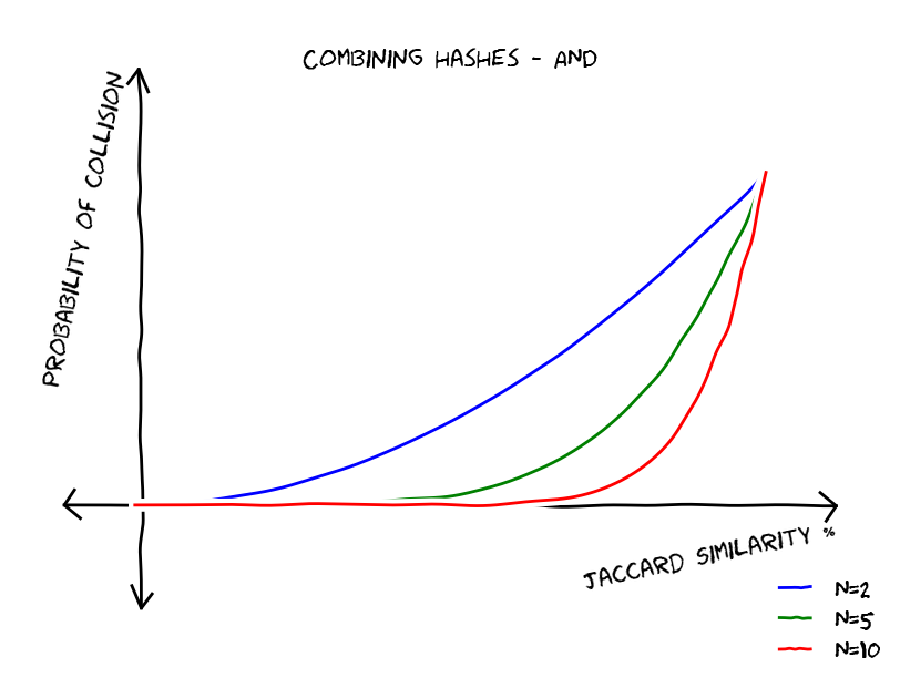
What if we accept a near duplicate if there is at least one chunk collision? The probability of none chunk colliding is , then the probability that at least one chunk collides is equal to . This gives us the following type of functions, these functions reduce false negatives but increase false positives.

As we said AND combinations (all collisions) reduce false positives and OR combinations (at least one collision) reduce false negatives, the ideal is to get a hash strategy that reduces both false positives and false negatives, if we manage to do so, we will get a graph similar to the first one. 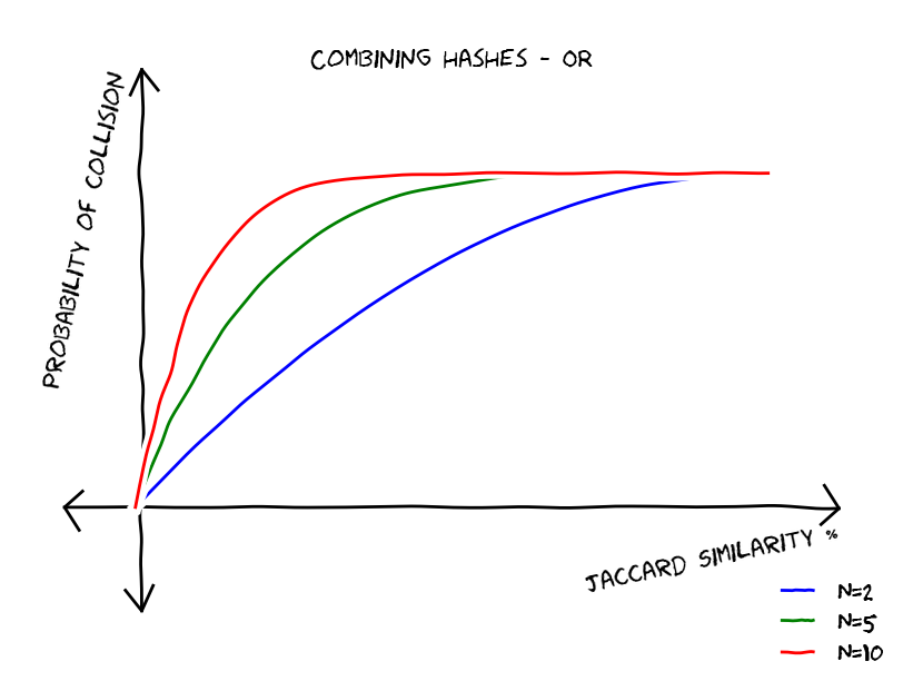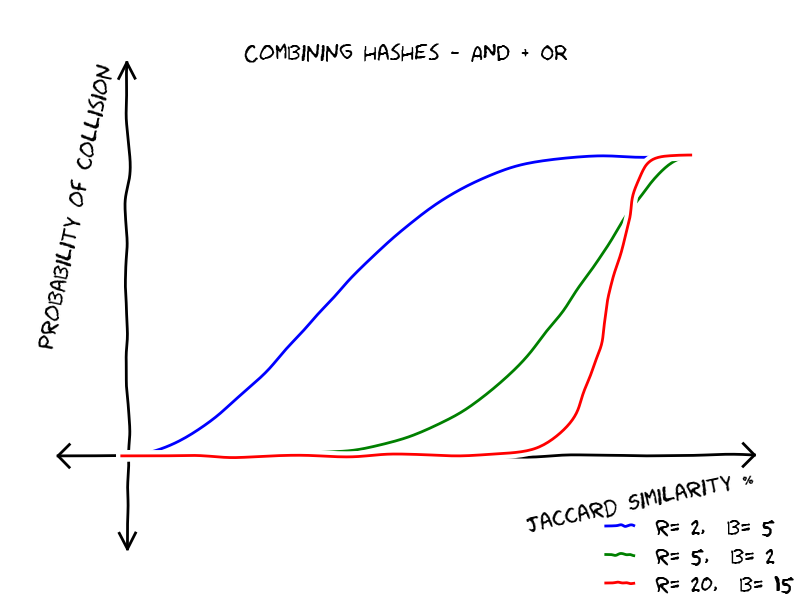The idea is straight-forward use both AND and OR combinations of hash functions, lets imagine that we have AND combinations followed by OR combinations. What does this mean? We break our files into chunks, lets say we have bands and each band has rows (or chunks). We hash each row using minhashing, we say that there is a collision in a particular band if each row in that band collide with the corresponding row from the same band in another file. If there is at least one band collision then we have a near duplicate. Lets see now how this procedure affects the collision probabilities. There is a collision in a particular band if all rows collide, therefore the probability for collision in that band is equal to . 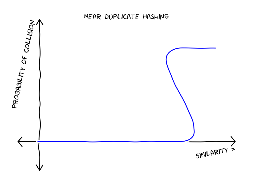The probability of having zero band collisions is equal to , this makes the probability of having at least one band collision equal to . This gives the following graphs:

As you can see, the more combinations we do the more we reach to the desired hash funcion that resembles a step function that accepts as near duplicates those pairs that have similarity larger than a threshold. On the efficiency of this method: all we need to do is to run through all our files and generate hashes, then based on these hashes we can generate a list of files that collide in at least one band, and this list is our near duplicates, but using this technique we avoided to compare each file with each file, making the algorithm linear in the number of files and suitable deduplicating large amounts of data.

References
[1] Rajaraman, A.; Ullman, J. (2010). “Mining of Massive Datasets, Ch. 3.”.

 

This is my first blog post. The purpose of this blog is to share knowledge in the areas of Data Mining, Data Science, Databases, and Machine Learning, I will try to add interesting posts in a regular basis (e.g. 1 post per week or 2 weeks)!